Capítulo 6 VARIABLES EN EL TIEMPO, AJUSTE A MODELO LINEAL Y ESTACIONARIO

6.1 Modelo lineal

plot(Indice_ts, main="Índice en el tiempo", xlab="Tiempo", ylab="Índice")
abline(reg = lm(Indice_ts ~ time(Indice_ts)))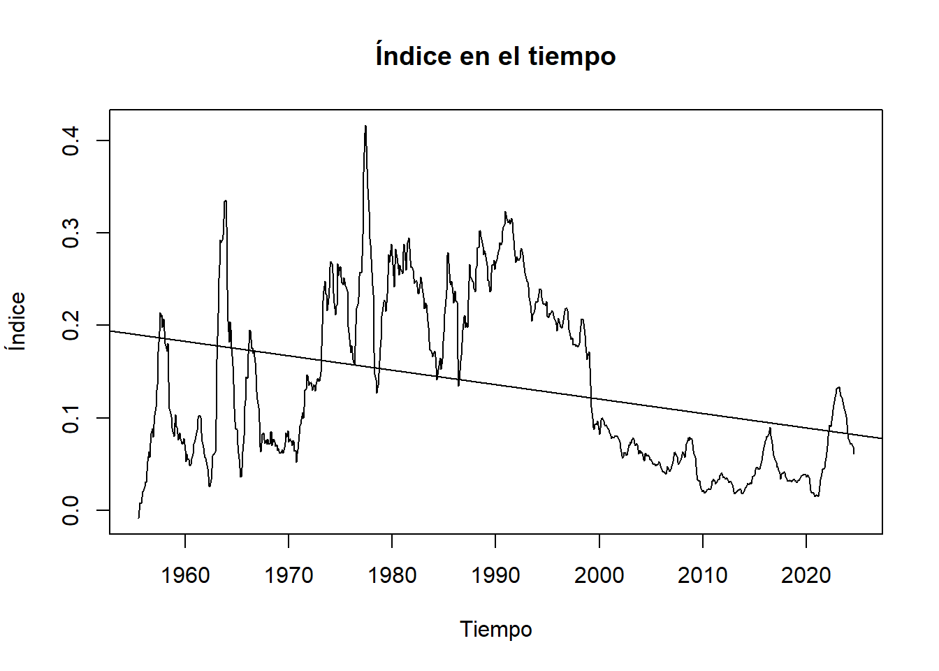

cycle(Indice_ts)

##      Jan Feb Mar Apr May Jun Jul Aug Sep Oct Nov Dec
## 1955                           7   8   9  10  11  12
## 1956   1   2   3   4   5   6   7   8   9  10  11  12
## 1957   1   2   3   4   5   6   7   8   9  10  11  12
## 1958   1   2   3   4   5   6   7   8   9  10  11  12
## 1959   1   2   3   4   5   6   7   8   9  10  11  12
## 1960   1   2   3   4   5   6   7   8   9  10  11  12
## 1961   1   2   3   4   5   6   7   8   9  10  11  12
## 1962   1   2   3   4   5   6   7   8   9  10  11  12
## 1963   1   2   3   4   5   6   7   8   9  10  11  12
## 1964   1   2   3   4   5   6   7   8   9  10  11  12
## 1965   1   2   3   4   5   6   7   8   9  10  11  12
## 1966   1   2   3   4   5   6   7   8   9  10  11  12
## 1967   1   2   3   4   5   6   7   8   9  10  11  12
## 1968   1   2   3   4   5   6   7   8   9  10  11  12
## 1969   1   2   3   4   5   6   7   8   9  10  11  12
## 1970   1   2   3   4   5   6   7   8   9  10  11  12
## 1971   1   2   3   4   5   6   7   8   9  10  11  12
## 1972   1   2   3   4   5   6   7   8   9  10  11  12
## 1973   1   2   3   4   5   6   7   8   9  10  11  12
## 1974   1   2   3   4   5   6   7   8   9  10  11  12
## 1975   1   2   3   4   5   6   7   8   9  10  11  12
## 1976   1   2   3   4   5   6   7   8   9  10  11  12
## 1977   1   2   3   4   5   6   7   8   9  10  11  12
## 1978   1   2   3   4   5   6   7   8   9  10  11  12
## 1979   1   2   3   4   5   6   7   8   9  10  11  12
## 1980   1   2   3   4   5   6   7   8   9  10  11  12
## 1981   1   2   3   4   5   6   7   8   9  10  11  12
## 1982   1   2   3   4   5   6   7   8   9  10  11  12
## 1983   1   2   3   4   5   6   7   8   9  10  11  12
## 1984   1   2   3   4   5   6   7   8   9  10  11  12
## 1985   1   2   3   4   5   6   7   8   9  10  11  12
## 1986   1   2   3   4   5   6   7   8   9  10  11  12
## 1987   1   2   3   4   5   6   7   8   9  10  11  12
## 1988   1   2   3   4   5   6   7   8   9  10  11  12
## 1989   1   2   3   4   5   6   7   8   9  10  11  12
## 1990   1   2   3   4   5   6   7   8   9  10  11  12
## 1991   1   2   3   4   5   6   7   8   9  10  11  12
## 1992   1   2   3   4   5   6   7   8   9  10  11  12
## 1993   1   2   3   4   5   6   7   8   9  10  11  12
## 1994   1   2   3   4   5   6   7   8   9  10  11  12
## 1995   1   2   3   4   5   6   7   8   9  10  11  12
## 1996   1   2   3   4   5   6   7   8   9  10  11  12
## 1997   1   2   3   4   5   6   7   8   9  10  11  12
## 1998   1   2   3   4   5   6   7   8   9  10  11  12
## 1999   1   2   3   4   5   6   7   8   9  10  11  12
## 2000   1   2   3   4   5   6   7   8   9  10  11  12
## 2001   1   2   3   4   5   6   7   8   9  10  11  12
## 2002   1   2   3   4   5   6   7   8   9  10  11  12
## 2003   1   2   3   4   5   6   7   8   9  10  11  12
## 2004   1   2   3   4   5   6   7   8   9  10  11  12
## 2005   1   2   3   4   5   6   7   8   9  10  11  12
## 2006   1   2   3   4   5   6   7   8   9  10  11  12
## 2007   1   2   3   4   5   6   7   8   9  10  11  12
## 2008   1   2   3   4   5   6   7   8   9  10  11  12
## 2009   1   2   3   4   5   6   7   8   9  10  11  12
## 2010   1   2   3   4   5   6   7   8   9  10  11  12
## 2011   1   2   3   4   5   6   7   8   9  10  11  12
## 2012   1   2   3   4   5   6   7   8   9  10  11  12
## 2013   1   2   3   4   5   6   7   8   9  10  11  12
## 2014   1   2   3   4   5   6   7   8   9  10  11  12
## 2015   1   2   3   4   5   6   7   8   9  10  11  12
## 2016   1   2   3   4   5   6   7   8   9  10  11  12
## 2017   1   2   3   4   5   6   7   8   9  10  11  12
## 2018   1   2   3   4   5   6   7   8   9  10  11  12
## 2019   1   2   3   4   5   6   7   8   9  10  11  12
## 2020   1   2   3   4   5   6   7   8   9  10  11  12
## 2021   1   2   3   4   5   6   7   8   9  10  11  12
## 2022   1   2   3   4   5   6   7   8   9  10  11  12
## 2023   1   2   3   4   5   6   7   8   9  10  11  12
## 2024   1   2   3   4   5   6   7   8

plot(aggregate(Indice_ts,FUN=mean))

boxplot(Indice_ts~cycle(Indice_ts))

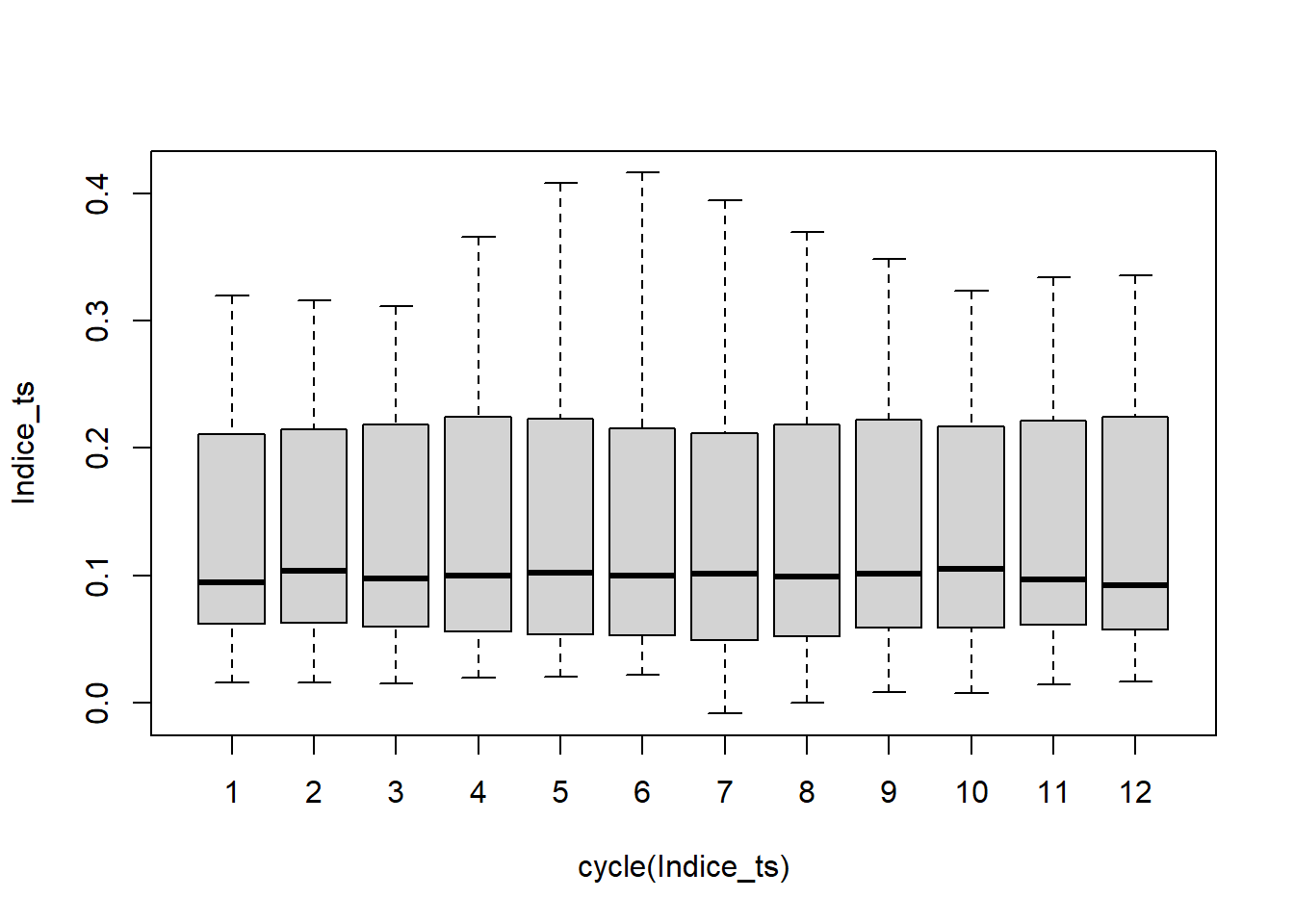Se observan valores homegéneos en los meses y no se observan valores atípicos marcados.

6.2 Modelo ARIMA

library(uroot)
ocb_test <- ocsb.test(Indice_ts)
print(ocb_test)

## 
##  OCSB test
## 
## data:  Indice_ts
## 
## Test statistic: -51.3138, 5% critical value: -1.803
## alternative hypothesis: stationary
## 
## Lag order 0 was selected using fixed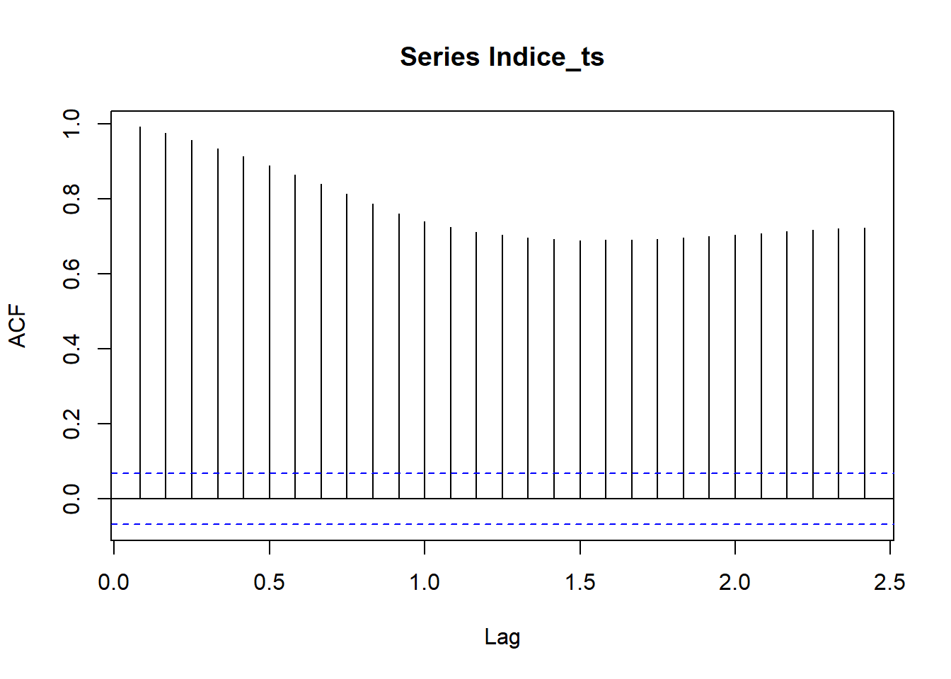

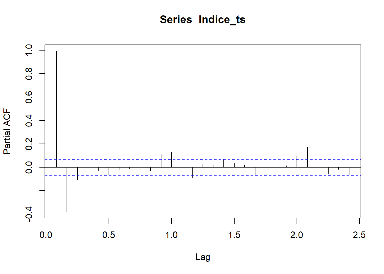
acf(Indice_ts)

pacf(Indice_ts)

El componente estacional de Indice_ts no es significativo, debido a esto se aplicará el modelo ARIMA directamente.

Indice_ts_diff <- diff(Indice_ts)
resultado_adf_diff <- adf.test(Indice_ts_diff, alternative = "stationary") 

modelo_arima <- auto.arima(Indice_ts_diff)  
summary(modelo_arima)

## Series: Indice_ts_diff 
## ARIMA(2,0,1)(0,0,2)[12] with zero mean 
## 
## Coefficients:
##          ar1     ar2     ma1     sma1    sma2
##       0.1628  0.3147  0.3815  -0.8884  0.0833
## s.e.  0.2118  0.1230  0.2159   0.0373  0.0375
## 
## sigma^2 = 5.259e-05:  log likelihood = 2903.25
## AIC=-5794.5   AICc=-5794.4   BIC=-5766.18
## 
## Training set error measures:
##                        ME      RMSE         MAE MPE MAPE      MASE        ACF1
## Training set 4.972306e-05 0.0072301 0.004844645 NaN  Inf 0.3930951 0.003467245

6.2.1 Test de residuos, AFC y PACF

Box.test(residuals(modelo_arima), type="Ljung-Box")

## 
##  Box-Ljung test
## 
## data:  residuals(modelo_arima)
## X-squared = 0.010002, df = 1, p-value = 0.9203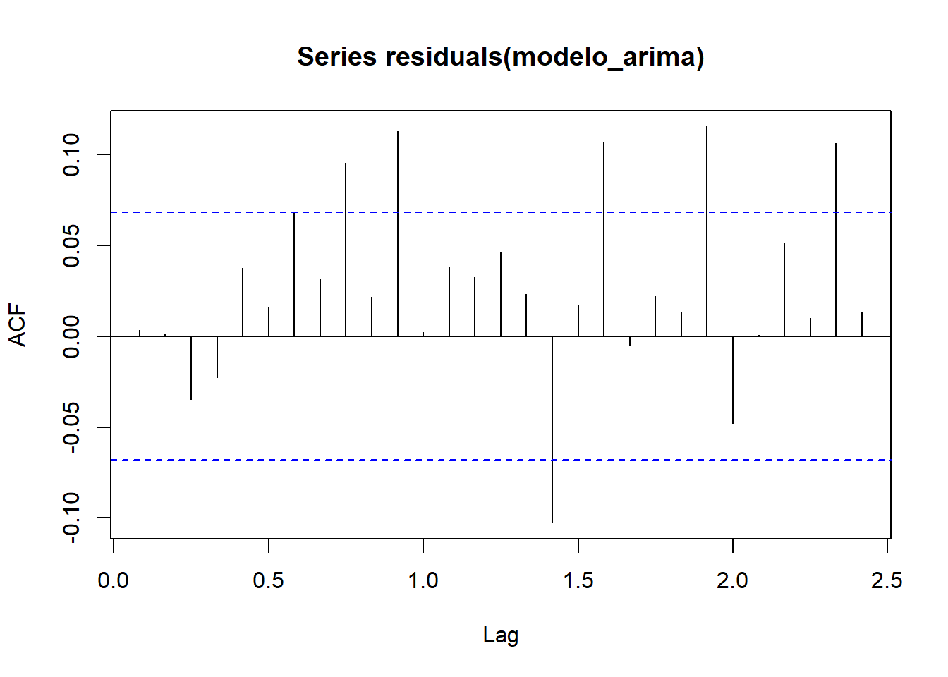

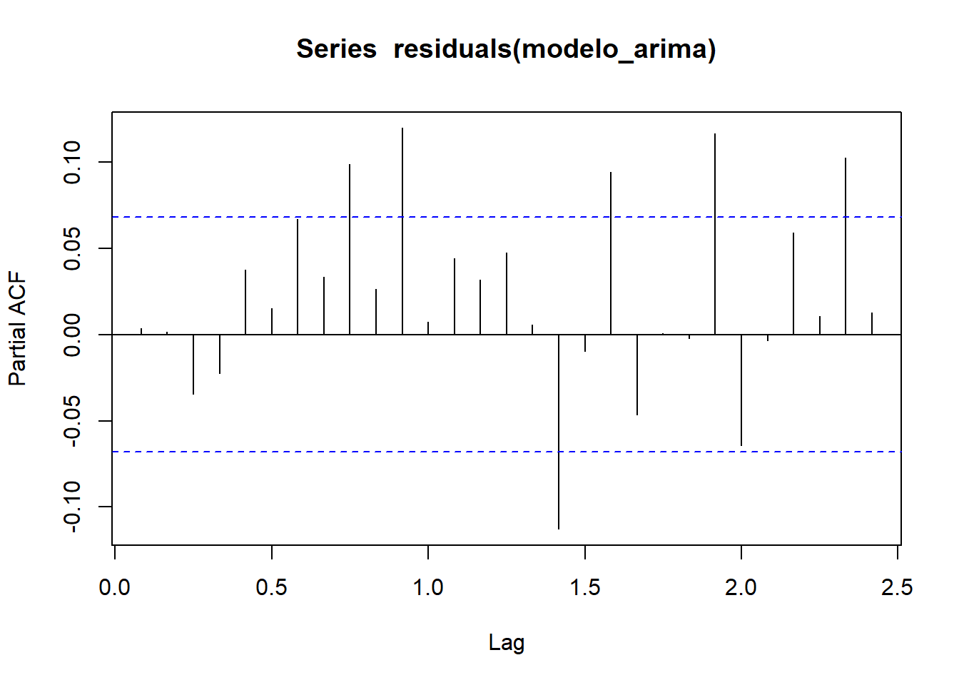
acf(residuals(modelo_arima))

pacf(residuals(modelo_arima))

De acuerdo con los resultados obtenidos, el p-value es mayor que 0.05, por lo que los residuales se pueden considerar como ruido blanco y el modelo representa bien la estructura de la serie de tiempo.

6.2.2 Pronóstico

forecast_data <- forecast::forecast(modelo_arima, h = 12)
plot(forecast_data, main = "Pronóstico del Índice")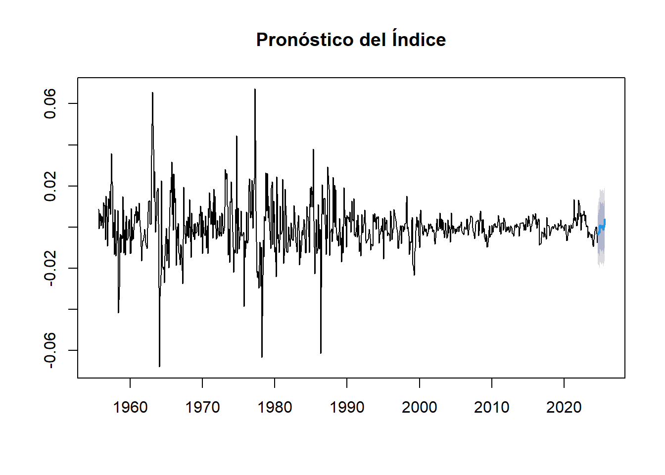

plot(forecast_data, main = "Pronóstico del Índice", xlab = "Año", ylab = "Indice_ts_diff", xlim = c(2015, 2025))
grid()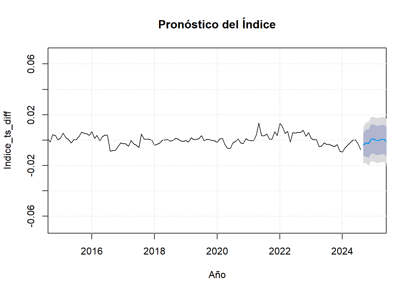

6.2.3 Resultados

residuales<-modelo_arima$residuals
qqnorm(residuales)
qqline(residuales)

checkresiduals(modelo_arima)

## 
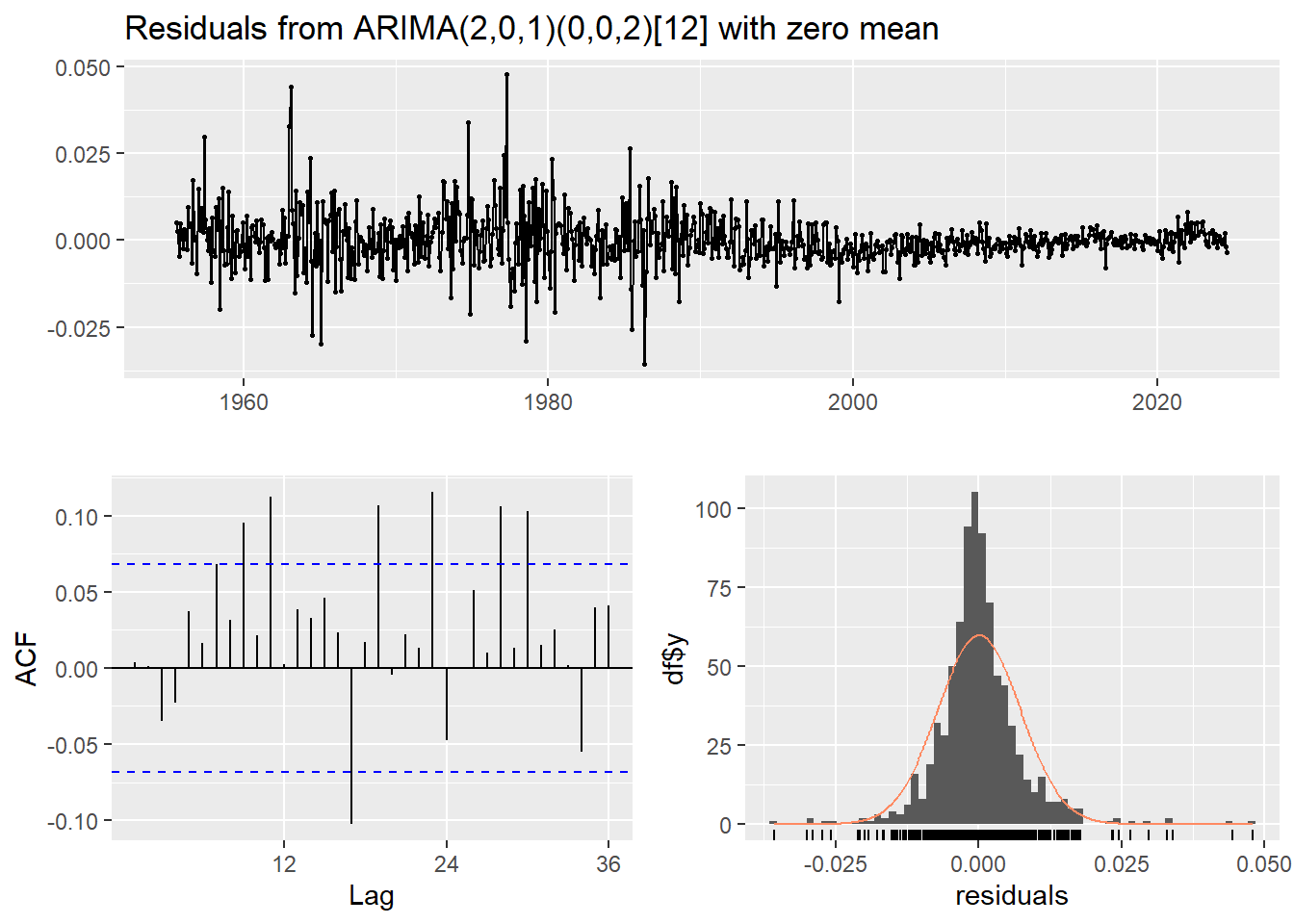
##  Ljung-Box test
## 
## data:  Residuals from ARIMA(2,0,1)(0,0,2)[12] with zero mean
## Q* = 63.564, df = 19, p-value = 1.043e-06
## 
## Model df: 5.   Total lags used: 24

shapiro.test(residuales)

## 
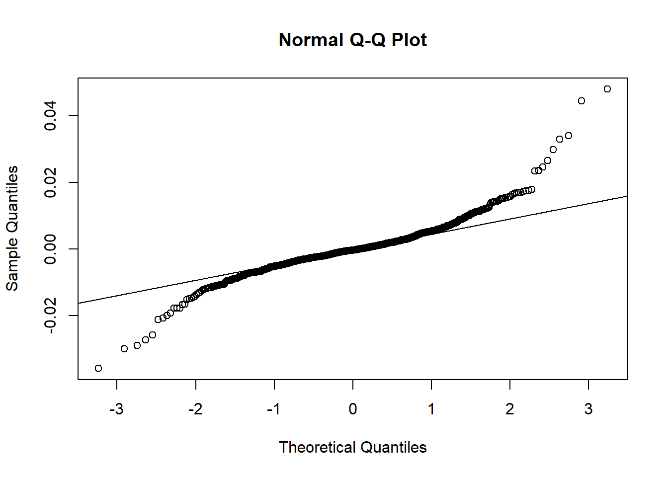
##  Shapiro-Wilk normality test
## 
## data:  residuales
## W = 0.91174, p-value < 2.2e-16

El valor de 0.91174 sugiere que los residuales están algo alejados de seguir una distribución normal, lo cual se confirma con el p-value bajo.

Box.test(residuales,type = "Ljung-Box")

## 
##  Box-Ljung test
## 
## data:  residuales
## X-squared = 0.010002, df = 1, p-value = 0.9203

El valor X-squared bajo, indica que hay poca correlación en los residuales y dado que el p-value es alto, significa que los residuales pueden ser considerados como ruido blanco.